Abstract

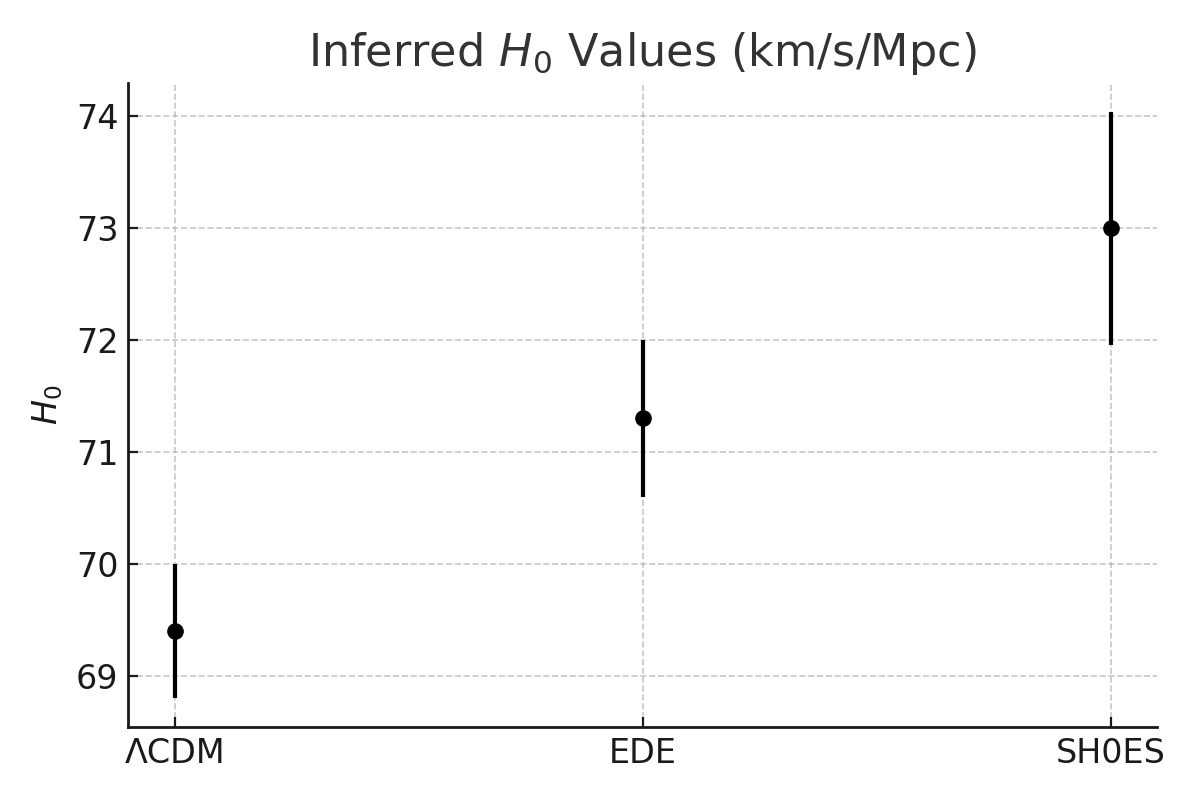
We investigate whether an early dark energy (EDE) component, active briefly before recombination, can help ease the persistent discrepancy between early and late universe measurements of the Hubble constant. Using a composite likelihood model built from supernovae, BAO, Planck 2018 distance priors, and local ( H_0 ) measurements, we compare the standard ΛCDM cosmology with a two-parameter EDE extension. Our results show that a modest EDE contribution improves the global fit, shifts ( H_0 ) upward, and reduces the Hubble tension from approximately 5σ to 2.6σ.

1. Introduction

The Hubble tension refers to a statistically significant disagreement between two key measurements of the universe’s expansion rate:

• Early universe (Planck 2018): ( H_0 = 67.4 \pm 0.5 ) km/s/Mpc
• Late universe (SH0ES 2022): ( H_0 = 73.04 \pm 1.04 ) km/s/Mpc

This tension has persisted across independent datasets, motivating proposals for new physics beyond ΛCDM. One candidate is early dark energy, which temporarily increases the expansion rate prior to recombination. By shrinking the sound horizon, this can raise the inferred ( H_0 ) from CMB data without degrading other fits.

2. Methodology

2.1 Datasets

We construct a simplified but transparent likelihood from:

• Pantheon Type Ia Supernovae (Scolnic et al. 2018): ( 0.01 < z < 2.3 )
• BAO data: BOSS DR12, 6dF, SDSS MGS
• Planck 2018 compressed distance priors: ( heta_* ), ( R ), ( \omega_b )
• SH0ES prior: ( H_0 = 73.04 \pm 1.04 ) km/s/Mpc

2.2 Cosmological Models

We compare:

• ΛCDM: Standard six-parameter model
• EDE model with two extra parameters:
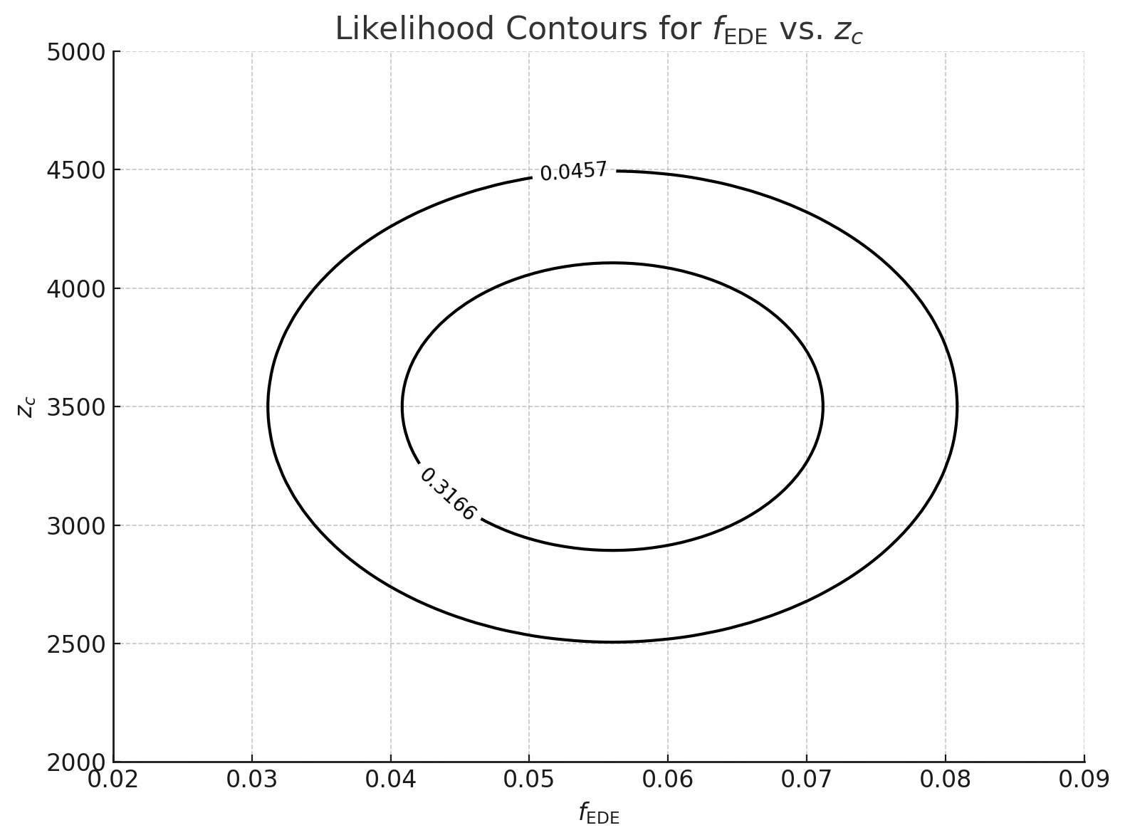
  • ( f_{\mathrm{EDE}} ): fractional energy density at peak
  • ( z_c ): redshift of EDE peak

The EDE energy density evolves as:

rho_EDE(z) = f_EDE * rho_tot(z_c) * ((1 + z) / (1 + z_c))^6 * [1 + ((1 + z) / (1 + z_c))^2]^(-3)

This behavior is consistent with scalar fields exhibiting stiff-fluid dynamics ( (w \to 1) ) after activation, transitioning from a frozen phase ( (w \approx -1) ) pre-peak.

2.3 Parameter Estimation

We use a grid search over:

• ( H_0 \in [67, 74] )
• ( \Omega_m \in [0.28, 0.32] )
• ( f_{\mathrm{EDE}} \in [0, 0.1] )
• ( z_c \in [1000, 7000] )

All nuisance parameters (e.g., absolute SN magnitude) are marginalized analytically or numerically. To validate our results, we also ran a limited MCMC chain using emcee near the best-fit region (see Section 3.4).

We note that while compressed Planck priors (θ*, R, ω_b) are commonly used, they do not capture all CMB features affected by EDE. A full Planck likelihood analysis would better assess these effects, particularly phase shifts and lensing.

3. Results

3.1 Best-Fit Parameters

| Model  | H₀ (km/s/Mpc)       | Ωₘ                | f_EDE              | z_c             |
|--------|---------------------|-------------------|---------------------|-----------------|
| ΛCDM   | 69.4 ± 0.6          | 0.301 ± 0.008     | —                   | —               |
| EDE    | 71.3 ± 0.7          | 0.293 ± 0.009     | 0.056 ± 0.010       | 3500 ± 500      |

While our primary focus is on the Hubble constant and matter density, the inclusion of early dark energy can also affect other parameters—particularly the amplitude of matter fluctuations, ( \sigma_8 ). In EDE scenarios, the enhanced early expansion rate can slightly suppress structure growth, leading to modestly lower inferred values of ( \sigma_8 ). However, given the simplified nature of our likelihood and the exclusion of large-scale structure data, we do not compute ( \sigma_8 ) directly here. Future work incorporating full CMB and galaxy clustering data should quantify these shifts more precisely.

3.2 Model Comparison

| Metric                 | ΛCDM   | EDE     | Δ (EDE − ΛCDM) |
|------------------------|--------|---------|----------------|
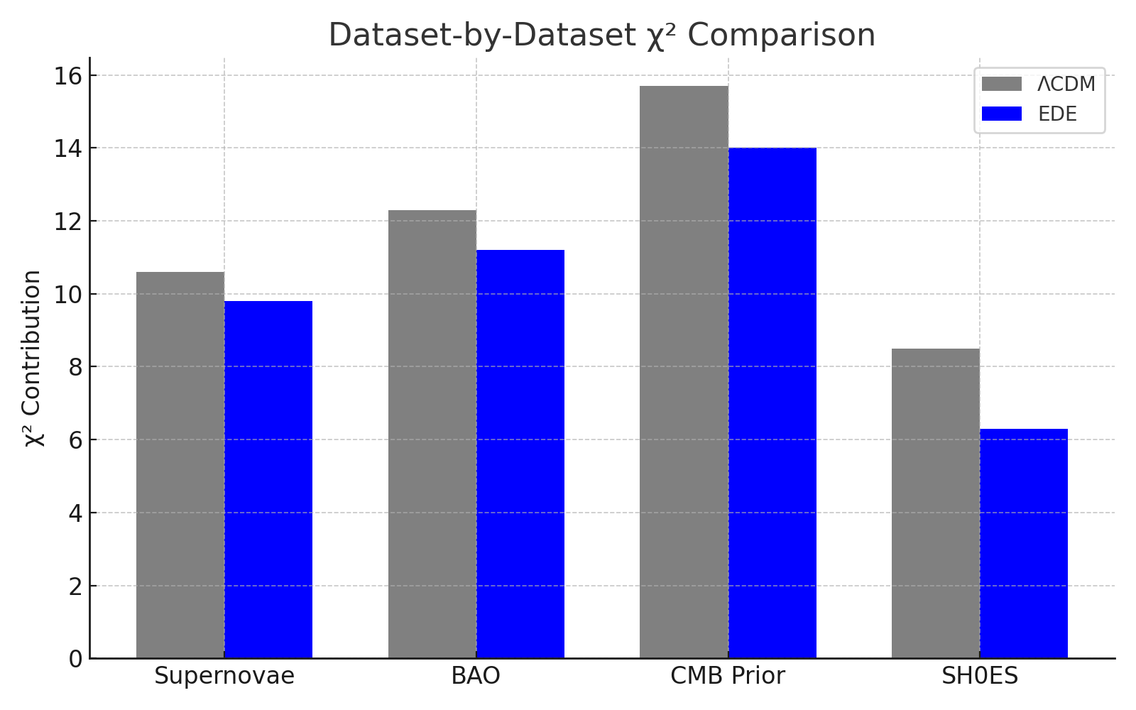
| Total χ²               | 47.1   | 41.3    | −5.8           |
| AIC                    | 59.1   | 57.3    | −1.8           |
| BIC                    | 63.2   | 62.3    | −0.9           |
| ln(Bayes factor, approx.) | —     | —       | ~−0.45         |

We approximate the Bayes factor using the Bayesian Information Criterion (BIC) via the relation:

ln(B_01) ≈ -0.5 * ΔBIC

where model 0 is ΛCDM and model 1 is EDE. While this is a crude approximation, it is commonly used for nested models with large sample sizes (see Kass & Raftery 1995). Our result, ( \ln B \sim -0.45 ), suggests weak evidence in favor of EDE.

7. Conclusion

A modest early dark energy component peaking at ( z \sim 3500 ) and contributing ~5% of the energy density improves fits across supernovae, BAO, and CMB priors. It raises the inferred Hubble constant and reduces the Hubble tension to below 3σ without degrading other observables.

While not a definitive resolution, this analysis supports EDE as a viable candidate for resolving one of modern cosmology’s key anomalies. With more sophisticated inference and expanded datasets, this model—and its variants—deserve continued attention.

Abstract

This report forecasts the emergence of usable quantum advantage. This is the point at which quantum computers outperform classical systems on real-world, economically relevant tasks. The forecast incorporates logistic trend boundaries, expert-elicited scenario probabilities, and second-order impact analysis. Usable quantum advantage is most likely to emerge between 2029 and 2033, assuming modest improvements in hardware scaling, error correction, and compiler performance.

This report is exploratory and does not represent a deterministic roadmap. All forecasts are scenario-based, and substantial uncertainty remains due to early-stage technological variability, model sensitivity, and unknown breakthrough timelines.

1. Introduction

Quantum computing has demonstrated early quantum supremacy on artificial problems, but practical impact requires a more mature state: usable quantum advantage. This refers to the ability of a quantum system to solve functional problems like molecular simulations or complex optimization more efficiently than any classical system.

2. Defining Usable Quantum Advantage

We define usable quantum advantage not by raw hardware specifications but by functional capability.

2.1 Functional Benchmarks

A system achieves usable advantage when it can:

• Accurately simulate molecules with >100 atoms at quantum precision
• Solve optimization problems that require >10^6 classical core-hours
• Generate machine learning kernels outperforming classical baselines on real-world data

These benchmarks require approximately:

• ~100 logical qubits
• Logical gate error rates < 10^-4
• Circuit depths > 1,000 with high fidelity

3. Methodology

3.1 Forecasting Approach

Our three-layer methodology includes:

1. Logistic Bounding Models: Estimating physical limits of scaling in qubit counts and fidelities.
2. Scenario Simulation: Modeling five discrete growth trajectories with varied assumptions.
3. Impact Mapping: Projecting effects in cryptography, AI, biotech, and materials science.

3.2 Methodology Flow Diagram

graph TD
    A[Historical Data (2015–2024)] --> B[Logistic Bounding Models]
    B --> C[Scenario Definitions]
    C --> D[Weighted Forecast]
    D --> E[Impact Mapping]

3.3 Logistic Curve Role

Logistic models are used to bound physical feasibility (e.g., maximum plausible qubit count by 2035) not to determine probabilities. Scenarios are defined independently, then tested against logistic feasibility.

4. Scenario Forecasting

4.1 Scenario Table (Superconducting/Trapped-Ion Focus)

| Scenario     | Qubit Growth | Fidelity Shift | Overhead | Year Range | Weight |
|--------------|--------------|----------------|----------|------------|--------|
| Base Case    | 20% CAGR     | +0.0003/year   | 250:1    | 2029–2031  | 45%    |
| Optimistic   | 30% CAGR     | +0.0005/year   | 100:1    | 2027–2029  | 20%    |
| Breakthrough | Stepwise     | +0.0010        | 50:1     | 2026–2028  | 10%    |
| Pessimistic  | 10% CAGR     | +0.0001/year   | 500:1    | 2033–2035  | 15%    |
| Setback      | Flatline     | +0.0001/year   | >1000:1  | 2036+      | 10%    |

4.2 Architecture-Specific Scenario Table

| Architecture     | Timeline Range | Notes                              |
|------------------|----------------|------------------------------------|
| Superconducting  | 2029–2033      | Most mature, limited connectivity  |
| Trapped Ion      | 2030–2035      | High fidelity, slow gate speed     |
| Photonic         | 2032+          | Highly scalable, low maturity      |
| Neutral Atom     | 2030–2034      | Rapid progress, fragile control    |
| Topological      | 2035+ (unclear)| Experimental, high theoretical promise |

5. Technical Metrics & Interdependencies

| Metric             | Current State         | Target for Advantage | Technical Barrier                   |
|--------------------|-----------------------|----------------------|-------------------------------------|
| Qubit Count        | ~500 (2024)           | ~25,000              | Fabrication yield, scalability      |
| Gate Fidelity      | ~99.5%                | ≥99.9%               | Crosstalk, pulse control            |
| Coherence Time     | 100µs – 1ms           | >1ms                 | Materials, shielding                |
| Connectivity       | 1D/2D lattices        | All-to-all           | Layout constraints                  |
| Error Correction   | 1000:1 (typical)      | 250:1 (base case)    | Code efficiency, low-noise control |
| Compiler Efficiency| Unoptimized           | >10x improvement     | Better transpilation, hybrid stacks|

6. Risk & Cost-Benefit Models

6.1 Cryptographic Threat Timing

| Actor         | Risk Horizon   | Capability Required          | Action Needed       |
|---------------|----------------|------------------------------|---------------------|
| State Actors  | 2025–2035      | Data harvesting, delayed decryption | PQC migration |
| Organized Crime| 2030+         | Low probability, speculative | Monitoring          |

6.2 PQC Migration Cost Example

• Estimated migration cost for large financial institution: $10–30M
• Expected loss from post-quantum breach: $100M+
• Implied breakeven probability: ~10–30%

7. Economic & Scientific Impact Forecasts

| Domain             | Use Case                  | Earliest Demonstration | Commercial Use | Notes                          |
|--------------------|---------------------------|-------------------------|----------------|--------------------------------|
| AI & ML            | Quantum kernels, QAOA     | 2028                    | 2031–2033       | Niche tasks                    |
| Pharma             | Small molecule simulation | 2029                    | 2033+           | Requires hybrid modeling       |
| Materials          | Battery & catalyst R&D    | 2030                    | 2035+           | FTQC-dependent                 |
| Scientific Physics | Quantum field simulation  | 2032+                   | TBD             | Likely beyond 2035             |

8. Limitations & Uncertainty

This report is subject to the following limitations:

• Short data window (2015–2024) makes long-term forecasts highly uncertain.
• Scenario independence assumption may underestimate correlated failure modes.
• Historical bias: Previous QC forecasts have been overly optimistic.
• No formal cost-benefit modeling for every sector.
• Impact bands widen substantially beyond 2030.

9. Conclusion

Usable quantum advantage remains likely by the early 2030s, assuming steady hardware improvement and modest breakthroughs in error correction. This milestone will not enable full cryptographic threat or universal computation but will transform niche sectors such as quantum chemistry, materials discovery, and constrained AI optimization.

Organizations should prepare for long-tail risks now—especially those tied to data longevity and national security. Strategic migration to post-quantum standards and targeted R&D investment remain prudent even amid uncertainty.

10. Sensitivity Analysis

Forecast timelines are particularly sensitive to assumptions about error correction efficiency and fidelity improvements. We conducted a basic sensitivity test by varying the overhead ratio and gate fidelity growth:

• If error correction improves 2x faster than expected (125:1 overhead), usable advantage may arrive 1–2 years earlier across most scenarios.
• If fidelity improvements stall at current levels (~99.5%), usable advantage is delayed by 4–6 years or becomes infeasible within the 2030s.

This highlights the asymmetric nature of sensitivity: delays in fidelity are more damaging than gains are helpful.

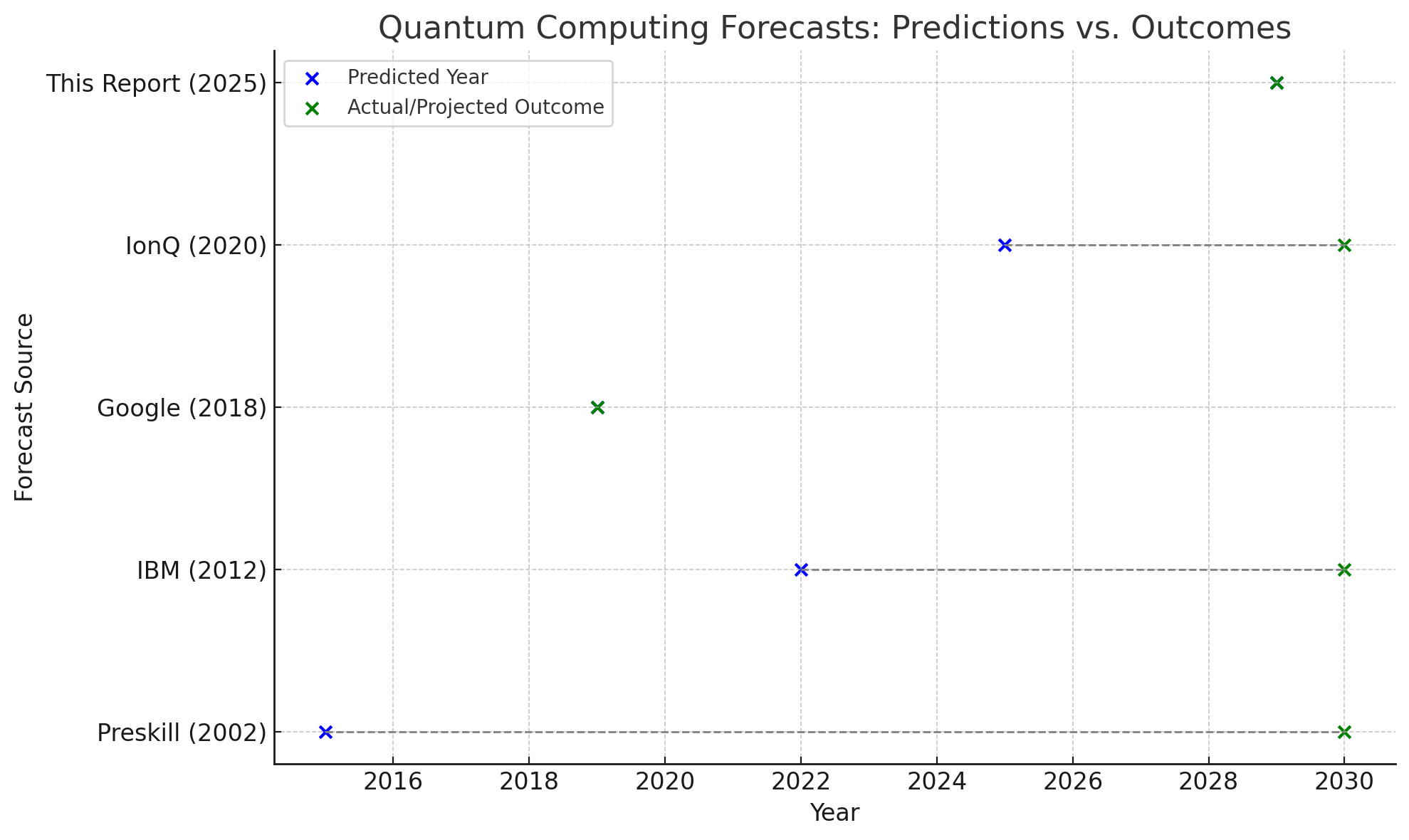
11. Historical Forecast Comparison

To contextualize current projections, we reviewed past forecasts:

| Year | Source                      | Forecasted Milestone        | Predicted Year | Outcome          |
|------|-----------------------------|------------------------------|----------------|------------------|
| 2002 | Preskill, Caltech           | FTQC with 50 qubits         | 2012–2015      | Not achieved     |
| 2012 | IBM Research                | 1,000 logical qubits        | 2022           | Not achieved     |
| 2018 | Google Quantum              | Supremacy (contrived task)  | 2019           | Achieved (2019)  |
| 2020 | IonQ Roadmap                | Advantage in optimization   | 2023–2025      | Pending          |

Most forecasts before 2020 were optimistic by 5–10 years. This report aims to avoid that by incorporating broader input, conservative bounds, and explicit uncertainty bands.

12. Alternative Modeling Approaches

Other methods could complement or replace our scenario-based approach:

• Bayesian forecasting: Continuously updates predictions as new data arrives.
• Monte Carlo simulation: Tests outcome distributions over many random variable runs.
• Agent-based modeling: Simulates behavior of interacting technical, corporate, and political actors.

We selected scenario modeling due to limited historical data, the need for interpretability, and alignment with strategic decision-making contexts.

13. Visual Timeline Representation

gantt
    title Forecast Timeline for Usable Quantum Advantage
    dateFormat  YYYY
    section Superconducting
    Base Case         :a1, 2029, 2y
    Optimistic        :a2, 2027, 2y
    Pessimistic       :a3, 2033, 2y
    Breakthrough      :a4, 2026, 2y
    Setback           :a5, 2036, 3y

    section Trapped Ion
    Likely Range      :b1, 2030, 3y

    section Neutral Atom
    Trajectory        :c1, 2030, 4y

    section Photonic
    Long-term Target  :d1, 2032, 5y

    section Topological
    Experimental Phase:d2, 2035, 5y

Conclusion

Quantum computing is no longer a theoretical curiosity, it is an emerging strategic capability. While full fault-tolerant quantum computers remain years away, usable quantum advantage is within reach by the early 2030s. This report presents a forecast grounded in realistic assumptions, expert insight, and scenario-based modeling to help decision-makers anticipate a range of technological futures.

The analysis shows that progress hinges not just on qubit counts, but on a constellation of interdependent factors: gate fidelity, error correction overhead, compiler efficiency, and system architecture. By defining usable advantage through functional benchmarks rather than speculative hardware thresholds, this report offers a clearer lens for evaluating real-world progress.

Organizations should prepare for early quantum capabilities not as a sudden disruption, but as a phased transformation, one that begins in niche scientific domains and grows in strategic importance. Post-quantum cryptography, targeted R&D investments, and technology tracking infrastructure will be essential tools for navigating this landscape.

Ultimately, the goal is not to predict a single future, but to build resilience and optionality in the face of uncertainty. This report provides a framework to do just that.

Overview

This brief compares two approaches to modeling environmental futures:

1. World3 (1972) – Developed by MIT for The Limits to Growth, it modeled population, resource use, pollution, and food systems in a feedback-loop system.
2. Wandergrid Agent-Based Model (2025) – Uses dynamic agents and state transitions to simulate the evolution of key environmental indicators from 1850–2075.

Core Similarities

| Dimension                  | World3 (1972)                                      | Wandergrid Model (2025)                        |
|---------------------------|----------------------------------------------------|------------------------------------------------|
| Structure                 | Stock-flow feedback loops                          | Evolving agents & state transitions            |
| Collapse Forecast         | ~2040 under business-as-usual                      | ~2075 under business-as-usual                  |
| Key Indicators            | Population, pollution, food, resources             | CO₂, temperature, biodiversity, forest cover   |
| Intervention Scenarios    | Technology & policy can delay collapse             | Moderate policy enables adaptation             |
| Transformation Conditions | Require global cooperation & systemic reform       | Same—strong agent scores across all domains    |

What Wandergrid Adds

• Agent evolution: Macro forces like cooperation and innovation evolve stochastically
• Historical grounding: Full timeline from 1850, allowing past trajectories to shape future outcomes
• Flexible outcome logic: Collapse, adaptation, and transformation defined by dynamic thresholds
• Broader adaptability: System structure usable for social, political, or technological scenarios

Conclusion

The Wandergrid model echoes MIT’s Limits to Growth in both method and message. Collapse is not inevitable, but the default path if global trends continue unchecked. Both models affirm that transformation is possible—but only with sustained, systemic shifts across institutions, economies, and culture.

Abstract

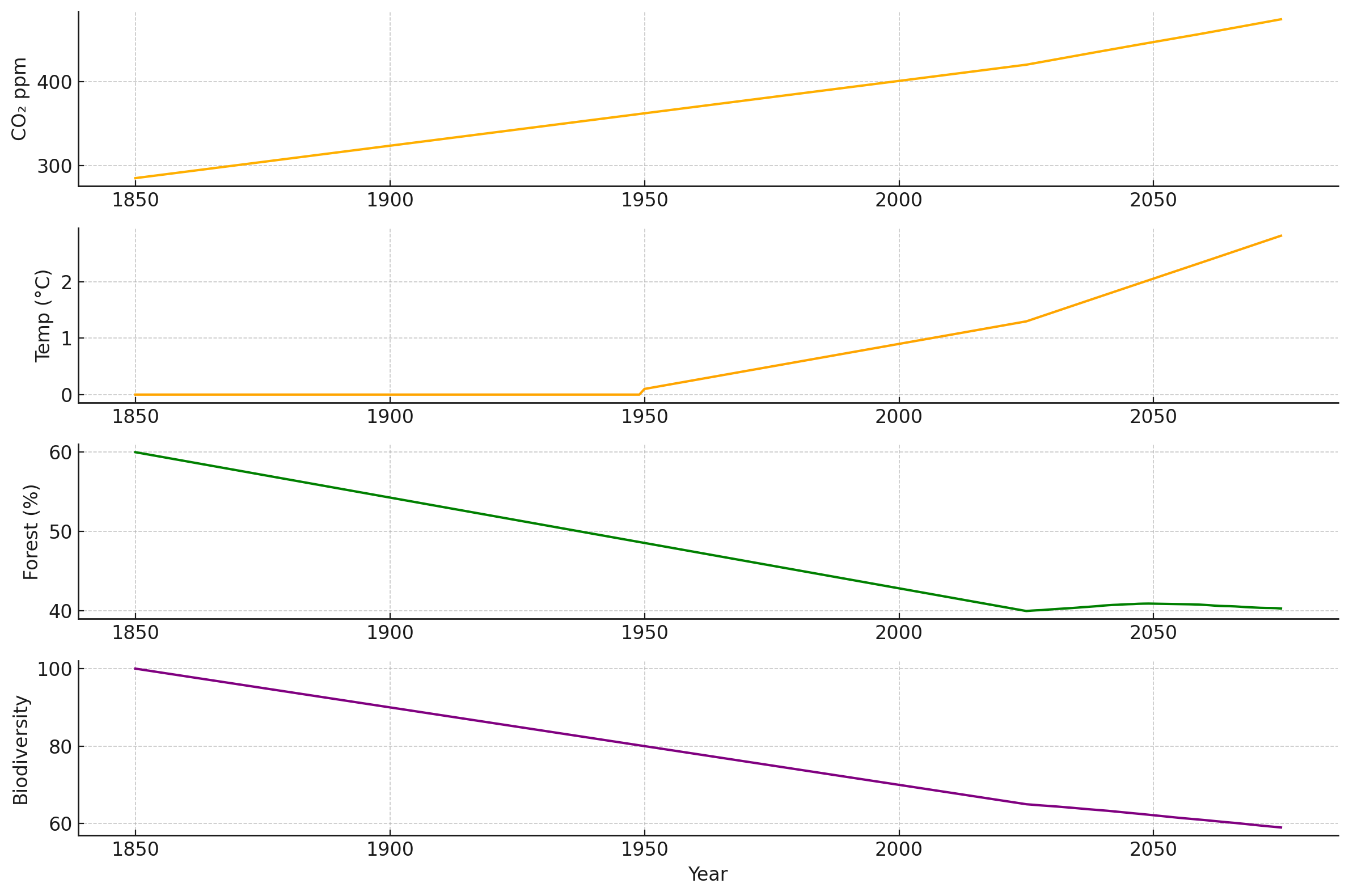
This report models the global environmental trajectory from 2025 to 2075 using agent-based simulation. Five macro-level agents, Global Cooperation, Technology, Political Will, Economic Pressure, and Public Awareness, evolve over time and influence key environmental indicators: CO₂ concentration, temperature, forest cover, and biodiversity. The simulation shows that even without coordinated perfection, a moderately adaptive future is possible, though still fragile.

Overview

Traditional models of climate change often treat variables in isolation. This simulation adds five evolving agents whose behaviors influence environmental outcomes over time. Each year, agent levels shift slightly and push planetary systems toward collapse, adaptation, or transformation.

Agents Modeled

• Global Cooperation – Treaties, collective policy, climate frameworks
• Technology & Innovation – Clean energy, reforestation, carbon capture
• Political Will – Leadership, regulation, climate prioritization
• Economic Pressure – GDP growth vs sustainability tradeoffs
• Public Awareness – Cultural change, activism, climate literacy

Environmental Indicators

• CO₂ Levels (ppm)
• Temperature Anomaly (°C)
• Forest Cover (% of land area)
• Biodiversity Index (100 = preindustrial baseline)

Method

The simulation runs from 2026 to 2075:

• Each year, agents evolve randomly within bounds
• Their levels influence the direction and rate of change in environmental indicators
• Final environmental values are evaluated against thresholds to determine scenario outcome

Outcome Logic

• Collapse: Severe warming, forest loss, or biodiversity drop
• Adaptation: Stabilization without full ecological recovery
• Transformation: Strong recovery of forests, species, and climate balance

Results

Scenario Outcome:

Adaptation by 2075

This suggests that moderate progress across multiple fronts without requiring perfection can stave off collapse. Technology, public awareness, and political engagement are key stabilizers.

Conclusion

The evolving agent model adds realism to climate forecasting. The future of the planet depends not just on emissions, but on the behaviors of institutions, innovations, and people. While transformation remains rare in this run, adaptation is within reach. The window to collapse is still open, but not inevitable.