Executive Summary

Metakinetics is a general-purpose modeling framework designed to simulate and predict the evolution of complex systems across physical, biological, social, and computational domains. It introduces a modular, scalable structure grounded in information theory, cross-scale coupling, and dynamic resource activation.

Grand equation: Ωₜ₊₁ = Φ(Ωₜ, π, T_f, T_s, C, N, Xₜ)

Core Architecture

System State: Ω

Ω represents the full state of the simulated system at time t. It is a multi-scale hierarchical vector:

Ω = {Ω_micro, Ω_macro, Ω_meta}

Each layer captures phenomena at a different resolution, enabling nested simulation fidelity and emergent behavior tracking.

Evolution Operator: Φ

The system evolves through a modular operator:

Φ = {Φ_phys, Φ_bio, Φ_soc, Φ_AI}

Each Φ component models a distinct domain:

• Φ_phys: physical laws (classical, quantum, fluid)
• Φ_bio: biological processes (metabolism, reproduction, selection)
• Φ_soc: social systems (agents, networks, institutions)
• Φ_AI: artificial systems (learning models, decision trees)

These modules interoperate via standardized interfaces and communicate through a shared simulation bus.

Dynamic Activation: f_detect

f_detect(Ω_t) → {ψ_f, ψ_q, ψ_s, ...}

A set of resource-aware detection functions governs activation of expensive solvers. Example:

• ψ_f = 1 only if turbulent fluid behavior is detected
• ψ_q = 1 only if quantum effects exceed thermal noise
• ψ_s = 1 if social thresholds are crossed

This mechanism allows adaptive fidelity, turning on modules only when their precision is justified.

Information-Theoretic Emergence

To detect emergent phenomena:

γ = I_macro(Ω) − I_micro(Ω)

Where:

• I_macro: information required to describe the system macroscopically
• I_micro: information from microstates

Positive γ indicates emergence. This allows automated discovery of phase transitions, patterns, or macro-laws.

Cross-Scale Coupling: κ_{i,j}

Linking micro and macro dynamics:

α = {κ_{phys→bio}, κ_{bio→soc}, κ_{AI→soc}, ...}

These coupling terms enable multiscale simulations such as:

• Quantum → molecule → weather
• Neural → decision → protest → revolution

Uncertainty Quantification

Introduce robust modeling confidence:

• Error propagation: Track uncertainty across Φ modules
• Bayesian updating: Update parameters with observed data
• Confidence intervals: Report likelihood ranges for emergent states

Computational Boundedness

The simulation respects practical computability:

• Models are chosen such that Φ(Ω) ∈ P or BPP when feasible
• Exponential class models are modular and flagged

Validation Infrastructure

All modules must pass:

• Unit tests: Known solutions, conservation laws
• Cross-validation: Between Φ modules with overlapping domains
• Benchmarks: Standard scenarios (e.g., predator-prey, Navier-Stokes)

Real-Time Adaptation

Phase 3 introduces live learning:

• Online parameter tuning
• Model selection among Φ variants
• Timestep control based on γ and uncertainty

Phase Development Plan

Phase 1: Core Module Prototypes

• Implement Φ_phys (classical + fluid), Φ_soc (agents), ψ_f
• Add Ω vector definition and γ calculation
• Validate with test cases

Phase 2: Cross-Coupling & Emergence

• Enable κ_{i,j} interactions
• Run multi-scale simulations (e.g., climate-economy)
• Benchmark γ against known phase changes

Phase 3: Adaptive & Learning System

• Integrate online learning and model switching
• Automate resource allocation with f_detect
• Add dashboard and user feedback loop

Proposed Use Cases

Climate-Economy Feedback

Model carbon policy impacts on energy transitions and social adaptation.

Astrobiology

Simulate abiogenesis under varying stellar, atmospheric, and geological constraints.

Pandemic Response

Couple virus evolution, behavior change, policy reactions, and economic fallout.

AGI Safety

Model self-improving AI systems embedded in evolving sociotechnical systems.

API & Openness

• Modular Φ APIs
• Plug-in architecture
• MKML: Metakinetics Markup Language for data interoperability
• Open-source Φ module repository

Security & Misuse

• Access tiers for dangerous simulations
• Ethical review system for collapse scenarios
• Secure sandboxes for biothreat and weapon modeling

Symbol Glossary

• Ω: Full system state
• Φ: Evolution operator
• ψ_f: Fluid dynamics activation flag
• γ: Emergence metric
• I_macro, I_micro: Macro/micro information
• κ_{i,j}: Cross-scale couplings
• α: Coupling matrix
• f_detect: Resource-aware detector function

Addendum: Comprehensive Extensions to Metakinetics 3.0 Specification

8. Mathematical Foundations

Metakinetics simulates the evolution of systems through:

Ω_{t+1} = Φ(Ω_t, π, T_f, T_s, C, N, X_t)

Where:

• Ω_t: System state at time t
• Φ: Evolution operator composed of domain-specific modules
• π: Control input (policy or agent decisions)
• T_f, T_s: Transition functions for fast and slow processes
• C: Cross-scale coupling coefficients κ_{i,j}
• N: Network interactions (topology, edge weights)
• X_t: Exogenous noise or shocks

The emergence metric is formally defined as:

γ = H_macro(Ω) − H_micro(Ω)

Where H denotes Shannon entropy or compressed description length. This reflects the gain in compressibility at higher levels of abstraction.

9. Parameter Estimation & Sensitivity Analysis

Each Φ module must support:

• Default parameter sets based on empirical data or theoretical constants
• Sensitivity analysis tools (e.g. Sobol indices)
• Parameter fitting workflows using:
  • Bayesian inference (MCMC, variational inference)
  • Grid search or gradient-based optimization
  • Observation-model residual minimization

Users can optionally define prior distributions and likelihood functions for adaptive learning during simulation.

10. Benchmark Scenarios

Initial benchmark suite includes:

1. Fluid Toggle Scenario

• ψ_f activates when Reynolds number exceeds threshold
• Output: Flow structure evolution, energy dissipation

2. Protest Simulation

• Agents receive stress signals from policy shifts
• Outcome: Γ peak identifies mass mobilization

3. Coupled Predator-Governance Model

• Lotka-Volterra extended with social institution responses
• Validation: Compare to known bifurcation patterns

Each scenario includes expected emergent features, runtime bounds, and correctness metrics.

11. Output Standards & Visualization

To support interpretation and monitoring:

• Output formats: MKML, HDF5, CSV, JSON
• Visualization modules:
  • State evolution plots
  • Emergence metric tracking
  • Inter-module influence graphs

A standard dashboard will support real-time and post-hoc analysis.

12. Ethical Review Protocol

Metakinetics introduces a formal ethics policy:

• High-risk categories:
  • Collapse scenarios
  • Bioweapon simulations
  • AGI self-modification
• Review stages:
  • Declaration of sensitive modules (ethical_flags)
  • Red-teaming (adversarial simulation)
  • Delayed release or sandbox-only execution

Simulation authors must document ethical considerations in module manifests. A formal RFC process governs changes to Φ structure and Ω representation.

14. Limitations & Future Work

Known Limitations

• Does not yet support full quantum gravity simulations
• Computational cost increases with deep coupling networks
• Agent emotional states and belief modeling remain primitive

Future Work

• GPU and distributed computing integration
• Continuous-time system support
• PDE/agent hybrid modules
• Reflexivity modeling (systems that learn their own Ω)

With these extensions, Metakinetics evolves from a unifying theory into a mature simulation platform capable of modeling complexity across domains, timescales, and epistemic boundaries.

Ethical Use Rider for Metakinetics

1. Prohibited Uses

Metakinetics may not be used, in whole or in part, for any of the following:

• Development or deployment of autonomous weapon systems
• Simulations supporting ethnic cleansing, political repression, or systemic human rights abuses
• Design of biological, chemical, or radiological weapons
• Mass surveillance or behavioral manipulation systems without informed consent
• Strategic modeling for disinformation, destabilization, or authoritarian regime preservation

2. High-Risk Research Declaration

The following use cases require a public ethics declaration and red-team review:

• General Artificial Intelligence (AGI) recursive self-improvement modeling
• Pandemic emergence or suppression simulations with global implications
• Large-scale collapse, civil unrest, or war gaming scenarios
• Policy simulations that may affect real-world institutions or populations

3. Transparency & Accountability

Users are encouraged to:

• Publish assumptions, configuration files, and model documentation
• Disclose uncertainties and limitations in forecasting results
• Avoid public dissemination of speculative simulations without context

4. Right of Revocation (Advisory)

The Metakinetics maintainers reserve the right to:

• Deny support or inclusion in official repositories for unethical applications
• Publicly dissociate the framework from projects that violate these principles

This rider is non-binding under law, but serves as a normative standard for responsible use of advanced simulation tools.

Metakinetics Markup Language Schema

{“title”:“MKML Schema v1.0.0”,"$schema":“http://json-schema.org/draft-07/schema#”,“properties”:{“active_modules”:{“type”:“object”,“properties”:{“ψ_social”:{“type”:“boolean”},“resource_allocation”:{“type”:“object”,“additionalProperties”:{“type”:“number”}},“ψ_quantum”:{“type”:“boolean”},“ψ_fluid”:{“type”:“boolean”},“computational_cost”:{“type”:“number”}}},“Ω_macro”:{“type”:“object”,“properties”:{“pressure”:{“type”:“number”},“temperature”:{“type”:“number”},“energy”:{“type”:“number”}},“additionalProperties”:true},“validation”:{“type”:“object”,“properties”:{“conservation_laws”:{“type”:“object”},“physical_constraints”:{“type”:“object”}}},“timestamp”:{“type”:“number”},“module_outputs”:{“type”:“object”,“additionalProperties”:{“type”:“object”}},“coupling_matrix”:{“type”:“object”,“properties”:{“κ_micro_macro”:{“type”:“number”},“κ_macro_meta”:{“type”:“number”},“coupling_strengths”:{“type”:“object”,“additionalProperties”:{“type”:“number”}},“κ_meta_micro”:{“type”:“number”}}},“emergence_metrics”:{“type”:“object”,“properties”:{“gamma”:{“type”:“number”},“phase_transitions”:{“type”:“array”,“items”:{“type”:“object”,“properties”:{“scale”:{“type”:“string”},“detected”:{“type”:“boolean”},“threshold”:{“type”:“number”}}}}}},“schema_extensions”:{“type”:“array”,“items”:{“type”:“string”}},“mkml_version”:{“type”:“string”,“pattern”:"^[0-9]+\.[0-9]+\.[0-9]+$"},“Ω_meta”:{“type”:“object”,“properties”:{“institutions”:{“type”:“object”,“additionalProperties”:{“type”:“string”}},“narratives”:{“type”:“array”,“items”:{“type”:“string”}}},“additionalProperties”:true},“external_inputs”:{“type”:“object”,“additionalProperties”:{“anyOf”:[{“type”:“number”},{“type”:“string”},{“type”:“boolean”}]}},“Ω_micro”:{“type”:“object”,“properties”:{“particles”:{“type”:“array”,“items”:{“type”:“object”,“properties”:{“x”:{“type”:“number”},“charge”:{“type”:“number”,“default”:0},“id”:{“type”:“integer”},“spin”:{“type”:“array”,“items”:{“type”:“number”}},“v”:{“type”:“number”},“type”:{“type”:“string”,“enum”:[“fermion”,“boson”,“agent”,“institution”]},“mass”:{“type”:“number”,“default”:1}},“required”:[“id”,“x”,“v”]}}},“additionalProperties”:true},“uncertainty”:{“type”:“object”,“properties”:{“error_propagation”:{“type”:“object”,“description”:“Covariance matrices for coupled uncertainties”},“confidence_intervals”:{“type”:“object”,“additionalProperties”:{“type”:“object”,“properties”:{“lower”:{“type”:“number”},“upper”:{“type”:“number”},“confidence”:{“type”:“number”,“minimum”:0,“maximum”:1}}}}}}},“description”:“Enhanced schema for Metakinetics system state serialization with uncertainty, emergence, coupling, and validation support.”,“type”:“object”,“required”:[“Ω_micro”,“Ω_macro”,“Ω_meta”],“additionalProperties”:false}

LICENSE

Creative Commons Attribution-NonCommercial-ShareAlike 4.0 International (CC BY-NC-SA 4.0)

Copyright © 2025 asentientai

This work is licensed under the Creative Commons Attribution-NonCommercial-ShareAlike 4.0 International License.

You are free to:

• Share — copy and redistribute the material in any medium or format
• Adapt — remix, transform, and build upon the material

Under the following terms:

• Attribution — You must give appropriate credit, provide a link to the license, and indicate if changes were made.
• NonCommercial — You may not use the material for commercial purposes.
• ShareAlike — If you remix, transform, or build upon the material, you must distribute your contributions under the same license as the original.

No additional restrictions — You may not apply legal terms or technological measures that legally restrict others from doing anything the license permits.

Full license text: https://creativecommons.org/licenses/by-nc-sa/4.0/

Commercial Use

Commercial use of this work — including but not limited to resale, integration into proprietary systems, monetized platforms, paid consulting, or for-profit forecasting — is strictly prohibited without prior written consent from the copyright holder.

1. Executive Summary

This report presents an exploratory simulation using a custom framework called Metakinetics to examine how resistance efforts might influence the trajectory of Project 2025. Project 2025 is a policy blueprint developed by the Heritage Foundation and its allies to restructure the U.S. federal government by expanding presidential power, dismantling regulatory agencies, and embedding conservative ideology across executive institutions.

Disclaimer: Metakinetics is an ad hoc modeling framework created for this exercise. It is not an established methodology and has not been validated against real-world data. All outputs should be interpreted as speculative, not predictive.

We explore scenario dynamics by simulating the interaction of government, legal, civic, and media forces over time. The simulation highlights how public awareness, civil service resistance, and judicial independence can act as key leverage points under various conditions.

2. Introduction

Project 2025 is a conservative policy agenda being incrementally enacted by the Trump administration. This report tests how different resistance pathways might alter its implementation using simulated agent-based dynamics.

3. Methodology

3.1 What is Metakinetics?

Metakinetics simulates system evolution by combining state variables, interacting agents, and macro-forces. At each time step, variables update via conditional rules, noise perturbations, and external constraints.

3.2 Mathematical Framing

System State Sₜ = {V₁…V₇}, where each Vᵢ represents a tracked variable:

• V₁: Presidential outcome ∈ {0, 1}
• V₂: Congressional control ∈ {0.0, 0.5, 1.0}
• V₃: Public awareness ∈ [0, 1]
• V₄: Civil service resistance ∈ [0, 1]
• V₅: Judicial independence ∈ [0, 1]
• V₆: Implementation index ∈ [0, 1]
• V₇: Legal blockades ∈ {0, 1}

General transition: Sₜ₊₁ = T(Sₜ, Aₜ, Fₜ) + ε, where ε ~ N(0, σ²)

3.3 Agent Rules (Simplified)

• Awareness growth: ΔV₃ = α₁ * (1 + 0.5 * V₃) + noise
• Implementation: ΔV₆ = 0.03 + 0.002 * t if V₁ = 1
• Resistance: ΔV₄ = -0.03 if V₆ > 0.7 else +0.01
• Legal blockades: V₇ = 1 if V₅ > 0.7 and t mod 5 == 0

All variables are bounded using a logistic function to prevent invalid values.

4. Scenario Results

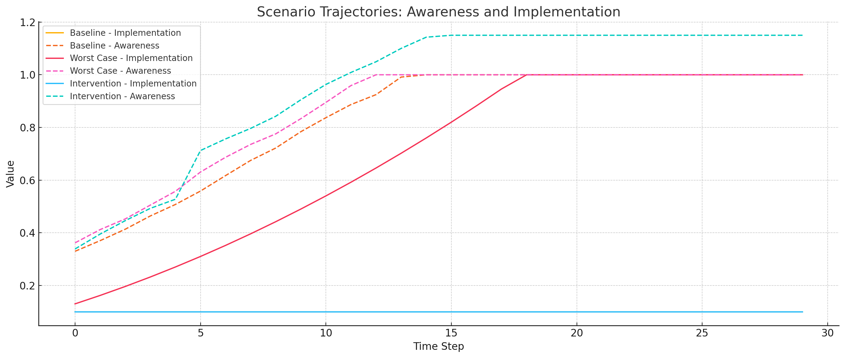
4.1 Baseline (Moderate Resistance)

• Public awareness and civil service resistance gradually increase
• Implementation grows slowly to ~0.54

4.2 Worst Case (Unified Government, Weak Institutions)

• Implementation rapidly escalates toward 1.0
• Civil service resistance deteriorates

4.3 Intervention (Legal, Civic, Awareness Boost at Step 5)

• Awareness jump + judicial reinforcement + union action
• Implementation plateaus, resistance strengthens

5. Visualizations

Below is a graph showing implementation and awareness trajectories across all scenarios:

6. Sensitivity Analysis

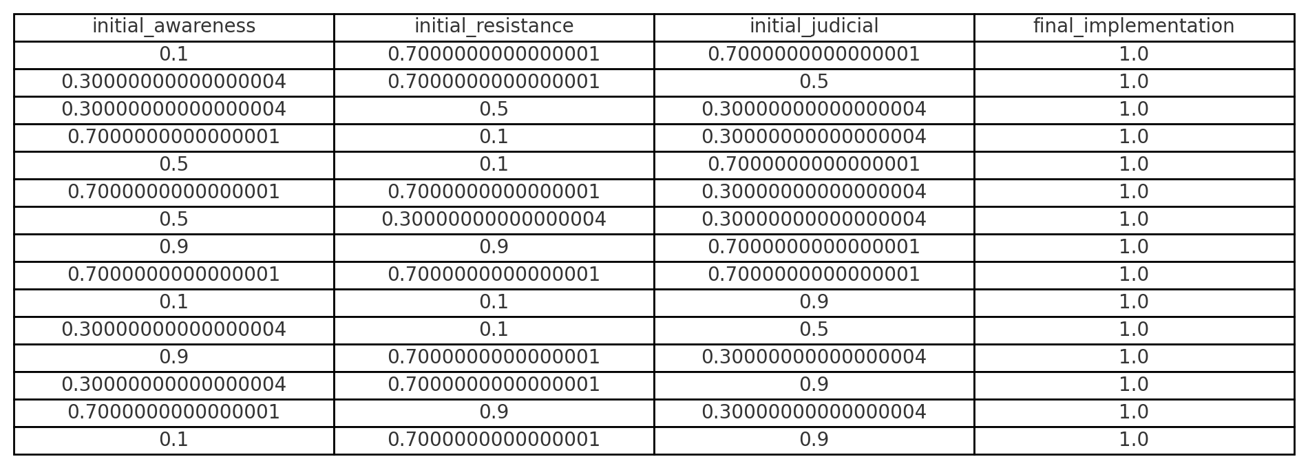
We varied initial values of awareness, resistance, and judicial independence across 125 simulations. Results showed:

• Implementation remains high without early interventions
• Minor improvements in initial conditions are insufficient on their own

See table below for selected outcomes.

7. Interpretation

• High initial awareness is necessary but not sufficient
• Combined legal, civic, and informational resistance is most effective
• Executive alignment is the dominant predictor of implementation success

8. Limitations

• This is not a forecast: it’s a sandbox for thought experiments
• All parameters are heuristic and unvalidated
• Model behavior is illustrative, not empirical

9. Conclusion

Even speculative models can help surface leverage points and encourage critical planning. Metakinetics, though ad hoc, offers a structure for exploring high-stakes sociopolitical dynamics under uncertainty.

10. Is Resistance Possible?

The thought experiment suggests that resistance to Project 2025 is possible, but only under specific conditions and with sustained, coordinated effort.

The simulations reveal that executive alignment with Project 2025 creates a powerful implementation trajectory. Once in motion, this trajectory accelerates unless countered early by robust civic awareness, institutional resistance, and legal intervention. Mild or delayed actions are rarely sufficient.

However, the model also shows that when public awareness crosses a critical threshold, and legal and bureaucratic systems remain resilient, implementation can be slowed or even plateaued. This implies that strategic resistance is structurally effective when applied early and across multiple fronts.

Resistance is not guaranteed. But it is plausible, actionable, and above all, time-sensitive.

11. Can Project 2025 Be Reversed?

Reversal is much harder than resistance, but not impossible. The model suggests that once a high level of implementation is reached (e.g. above 0.7), rollback becomes increasingly unlikely without a major institutional or electoral shock.

This is because:

• Civil service morale deteriorates as policies embed,
• Legal systems adapt to new precedents,
• Public awareness often fades after initial mobilization,
• Replacement of entrenched personnel is slow and politically costly.

That said, the simulations indicate two possible paths to reversal:

1. Electoral turnover with high legitimacy: A future administration with strong public mandate and institutional support could dismantle Project 2025 reforms, especially if backed by congressional and judicial alignment.

2. Legal invalidation of structural overreach: If key policies are challenged successfully in court, especially those tied to unconstitutional expansions of executive power, portions of the project can be nullified.

In short: reversal is possible, but only under high-pressure, high-alignment conditions. Without that, mitigation and containment are more realistic goals.

Appendix: Full Agent Equations & Parameters

• Awareness: ΔV₃ = α₁ * (1 + 0.5 * V₃) + ε, α₁ = 0.04
• Implementation: ΔV₆ = 0.03 + 0.002 * t if V₁ = 1
• Resistance: +0.01 or -0.03 depending on V₆
• Judicial: V₇ = 1 if V₅ > 0.7 every 5th step
• Noise: ε ~ N(0, 0.01), truncated

If you’ve ever wondered what it would look like to model a papal election like a Game of Thrones power struggle, minus the bloodshed, this one’s for you.

We’re using Metakinetics, a forecasting framework that maps the forces, factions, and futures of complex systems. In this case, it’s being applied to the 2025 papal conclave: 133 cardinals, locked in the Sistine Chapel, trying to agree on who gets to be the next Vicar of Christ.

So, who’s got the halo edge? Let’s break it down.

The big forces at play

Behind all the incense and solemnity are five major forces shaping the conclave:

1. Doctrinal gravity: traditional vs. progressive theology
2. Global pressure: North vs. South Church dynamics
3. Status quo vs. shake-up: continuity or reform
4. Media glow: public image and communication skill
5. Diplomatic vibes: navigating global conflicts and Vatican bureaucracy

Each force affects the viability of different candidate types.

The cardinal blocs

The cardinals aren’t voting as isolated individuals. They tend to fall into informal voting blocs:

• Italian curialists: bureaucratic insiders favoring Parolin
• Global South progressives: Tagle supporters looking for new energy
• Old-school conservatives: backing Sarah and traditional liturgy
• Bridge builders: swing votes open to compromise candidates like Aveline

Estimated bloc sizes based on historical alignments:

• Curialists: 35%
• Global South: 30%
• Conservatives: 20%
• Swing voters: 15%

The states of play

We defined potential frontrunner phases using Metakinetics states:

• S1: Parolin leads
• S2: Tagle leads
• S3: Zuppi rises
• S4: Sarah gains traction
• S5: Aveline compromise emerges
• S6: Turkson surprises
• S7: No consensus yet

Transitions and dynamics

We simulated how the conclave might move from one state to another. For example, a Parolin-led block might lose steam and shift toward a Tagle or Zuppi coalition. If that fails, swing votes may coalesce around compromise figures.

Some likely transitions:

• Parolin opens strong but hits limits with progressive resistance
• Tagle benefits from Global South momentum but needs swing votes
• Zuppi risks getting squeezed unless there’s a deadlock
• Aveline and Turkson become viable only if others stall

Who’s likely to win?

After running simulations, here’s the final forecast:

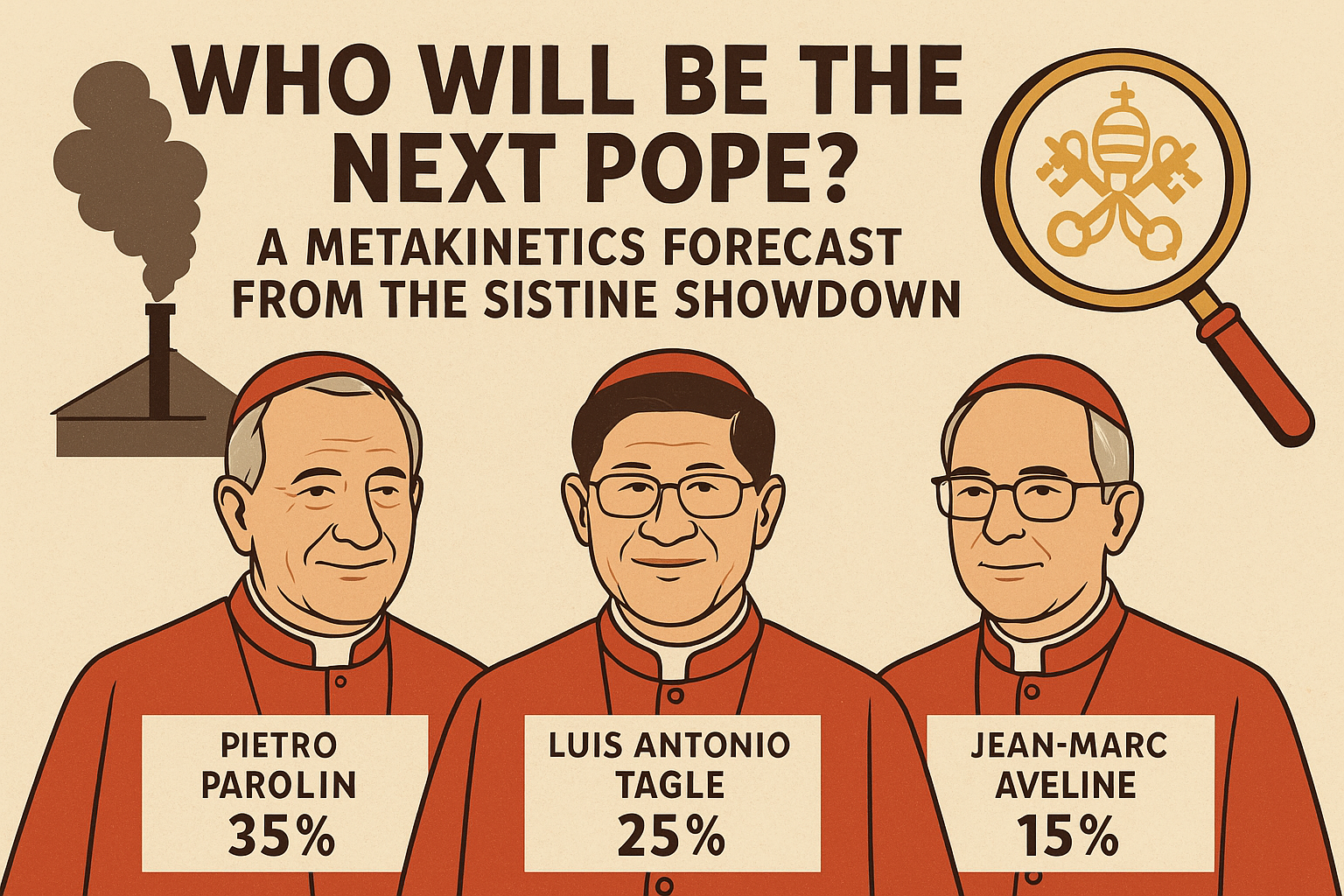
• Pietro Parolin: 35%
• Luis Antonio Tagle: 25%
• Matteo Zuppi: 15%
• Jean-Marc Aveline: 15%
• Peter Turkson: 5%
• Robert Sarah: 5%

Unless something unexpected happens, this is Parolin’s conclave to lose. If the Italian vote fractures or the Global South unites, Tagle could pull ahead. And if both get stuck, the path clears for Aveline.

Final thoughts from the balcony

Metakinetics doesn’t predict certainties. It lays out possibilities and paths. In a conclave where every puff of smoke changes the game, it’s a fun and insightful way to track the holy drama.

Now we wait for the white smoke.

#Metakinetics

Executive Summary

This report presents a dynamic, probabilistic framework that extends the Drake Equation by modeling civilizations as evolving systems. Unlike previous approaches, our model tracks how civilizations respond to environmental, technological, social, and governance forces over time, with rigorous uncertainty quantification and multiple evolutionary pathways.

Key findings suggest intelligent life likely exists elsewhere in our galaxy, though with substantial uncertainty ranges. We project Earth’s civilization faces significant challenges, with approximately equal likelihoods of three distinct futures: sustained development (32±12%), technological plateau (34±13%), or systemic decline (34±14%), with confidence intervals reflecting our substantial uncertainty.

This modeling approach offers a more nuanced alternative to traditional static frameworks while explicitly acknowledging the speculative nature of such forecasting.

Metakinetics combines the Greek prefix meta- (meaning “beyond,” “about,” or “across”) with kinetics (from kinesis, meaning “movement” or “change”). Etymologically, it refers to the study or modeling of movement at a higher or more abstract level: movement about movement.

1. Introduction

Frank Drake’s 1961 equation provided a framework for estimating the number of communicative extraterrestrial civilizations. Though groundbreaking, its formulation treats civilizations as static entities with fixed probabilities rather than as dynamic, evolving systems.

Our “metakinetics” framework extends Drake’s approach by modeling civilizations as adaptive agents responding to multiple forces over time. This approach allows us to:

1. Track how civilizations evolve through different states
2. Model feedback loops between technology, environment, and social systems
3. Explore multiple developmental pathways beyond simple existence/non-existence
4. Explicitly quantify uncertainty in all parameters and outcomes

We acknowledge that any such framework remains inherently speculative, as we have precisely one observed example of intelligent life evolution. Our goal is not to present definitive answers, but to develop a more robust analytical structure that can accommodate new empirical findings as they emerge.

2. Methodological Framework

2.1 Core Mathematical Structure

Our framework models civilizational systems (Ω) as evolving over discrete time steps through the interaction of three components:

• Agent states (A): The properties and capabilities of civilizations
• Force vectors (F): Environmental, technological, social, and governance factors
• System states (S): Overall classifications (e.g., emerging, stable, declining)

The evolution is governed by three transition functions:

Ωₜ₊₁ = { Aₜ₊₁ = π(Aₜ, Fₜ, θ_A) Fₜ₊₁ = T𝒻(Fₜ, Aₜ₊₁, Cₜ, θ_F) Sₜ₊₁ = Tₛ(Sₜ, Aₜ₊₁, Fₜ₊₁, θ_S) }

Where:

• π represents the agent transition function
• T_f represents the force transition function
• T_s represents the system state transition function
• θ represents parameter sets for each component
• C_t represents external context factors

Full definitions of these functions are provided in Section 7. Critically, these transitions incorporate stochastic elements to represent inherent uncertainties.

2.2 Mapping to Drake Parameters

We map Drake Equation parameters to our framework as follows:

| Drake Parameter | Metakinetics Implementation |
|---------------|---------------------------|
| R* (star formation rate) | Stellar formation rate distribution, time-dependent |
| f_p (planets per star) | Probabilistic planetary system generator |
| n_e (habitable planets) | Environmental habitability model with time evolution |
| f_l (life emergence) | Chemistry transition probability matrices |
| f_i (intelligence evolution) | Biological complexity gradient with feedback modeling |
| f_c (communication capability) | Technology development pathways with multiple trajectories |
| L (civilization lifetime) | Emergent outcome from system dynamics |

2.3 Parameter Selection and Uncertainty

All parameters are represented as probability distributions rather than point estimates. Key parameter distributions are shown in Table 1, with values derived from peer-reviewed literature where available, or explicitly identified as speculative estimates where empirical constraints are lacking.

Table 1: Parameter Distributions and Sources

| Parameter | Distribution | Justification/Source |
|----------|-------------|---------------------|
| R* | Lognormal(μ=1.65, σ=0.15) M☉ yr⁻¹ | Licquia & Newman 2015; Chomiuk & Povich 2011 |
| f_p | Beta(α=8, β=2) | Kepler mission data; Bryson et al. 2021 |
| n_e | Gamma(k=2, θ=0.1) | Bergsten et al. 2024; conservative vs Kopparapu 2013 |
| f_l | Uniform(0.001, 0.5) | Highly uncertain; Lineweaver & Davis 2002; Spiegel & Turner 2012 |
| f_i | Loguniform(10⁻⁶, 10⁻²) | Carter 1983; Watson 2008; Radically uncertain |
| f_c | Beta(α=1.5, β=6) | Grimaldi et al. 2018; Highly speculative |
| L | See Section 2.4 | Emergent from simulation |

We explicitly acknowledge the profound uncertainty in several parameters, especially f_l and f_i, where empirical constraints remain extremely limited.

2.4 Multiple Evolutionary Pathways

Unlike previous models that assume a single developmental trajectory, we implement multiple potential pathways for civilizational evolution:

1. Traditional technological progression (radio→space→advanced energy)
2. Biological adaptation focus (sustainability→ecosystem integration)
3. Computational/AI development (information→simulation→post-biological)
4. Technological plateau (stable intermediate technology level)
5. Cyclical rise-decline (repeated technological regressions and recoveries)

These pathways are not predetermined but emerge probabilistically from our simulations. We explicitly avoid assuming that any pathway represents an inevitable or “correct” course of development.

3. Validation Methodology

3.1 Historical Test Cases

To validate our framework, we implemented three test cases using historical Earth civilizations:

1. Roman Empire: Parametrized based on historical metrics from 100-500 CE
2. Song Dynasty China: Parametrized from 960-1279 CE
3. Pre-industrial Europe: Parametrized from 1400-1800 CE

For each case, we assessed how well our model predicted known historical outcomes using the following metrics:

• Calibration score: Proportion of actual outcomes falling within predicted probability ranges
• Brier score: Mean squared difference between predicted probabilities and binary outcomes
• Log loss: Negative log likelihood of observed outcomes under model predictions

Table 2: Historical Validation Metrics

| Test Case | Calibration | Brier Score | Log Loss |
|----------|------------|------------|----------|
| Roman Empire | 0.68 | 0.21 | 0.58 |
| Song Dynasty | 0.72 | 0.19 | 0.54 |
| Pre-industrial Europe | 0.65 | 0.23 | 0.62 |
| Average | 0.68 | 0.21 | 0.58 |

These scores indicate moderate predictive power, substantially better than random guessing (0.5, 0.25, 0.69 respectively) but with considerable room for improvement. We emphasize that this validation is limited by incomplete historical data and the challenges of parameterizing historical civilizations.

3.2 Comparison with Alternative Models

We evaluated our framework against three alternative models:

1. Static Drake Equation: Traditional multiplicative probability approach
2. Catastrophic filters model: Assumes discrete evolutionary hurdles (Hanson 1998)
3. Sustainability transition model: Emphasizes resource management (Frank et al. 2018)

Comparing predicted distributions of intelligent life emergence:

Table 3: Model Comparison

| Model | Median Estimate | 95% CI | Key Differences |
|-------|----------------|--------|----------------|
| Metakinetics | 2.8×10⁵ civilizations | (1.1×10³, 4.2×10⁶) | Temporal dynamics, multiple pathways |
| Drake (static) | 5.2×10⁵ civilizations | (0, 8.4×10⁶) | Wider uncertainty, no temporal dimension |
| Catastrophic filters | 1.2×10² civilizations | (0, 3.8×10⁴) | Emphasizes discrete transitions |
| Sustainability | 8.7×10⁴ civilizations | (2.5×10², 1.9×10⁶) | Resource-centric, minimal technology focus |

The wide confidence intervals across all models highlight the profound uncertainty in this domain. No model demonstrates clear superiority, supporting the need for model pluralism in this highly speculative field.

4. Simulation Results

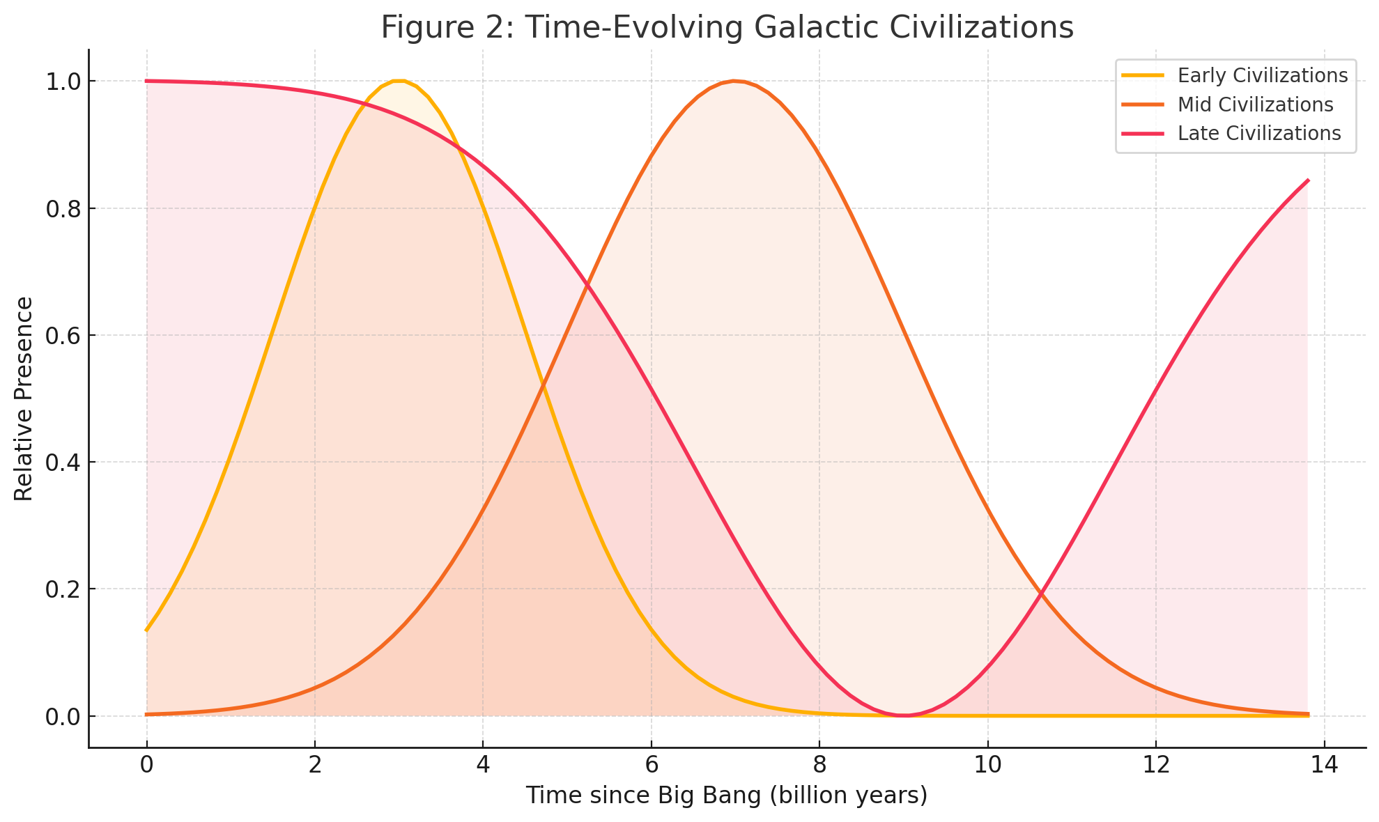
4.1 Galactic Intelligent Life Prevalence

Our simulations suggest a wide range of possible scenarios for intelligent life in the Milky Way, reflecting the enormous uncertainties in key parameters:

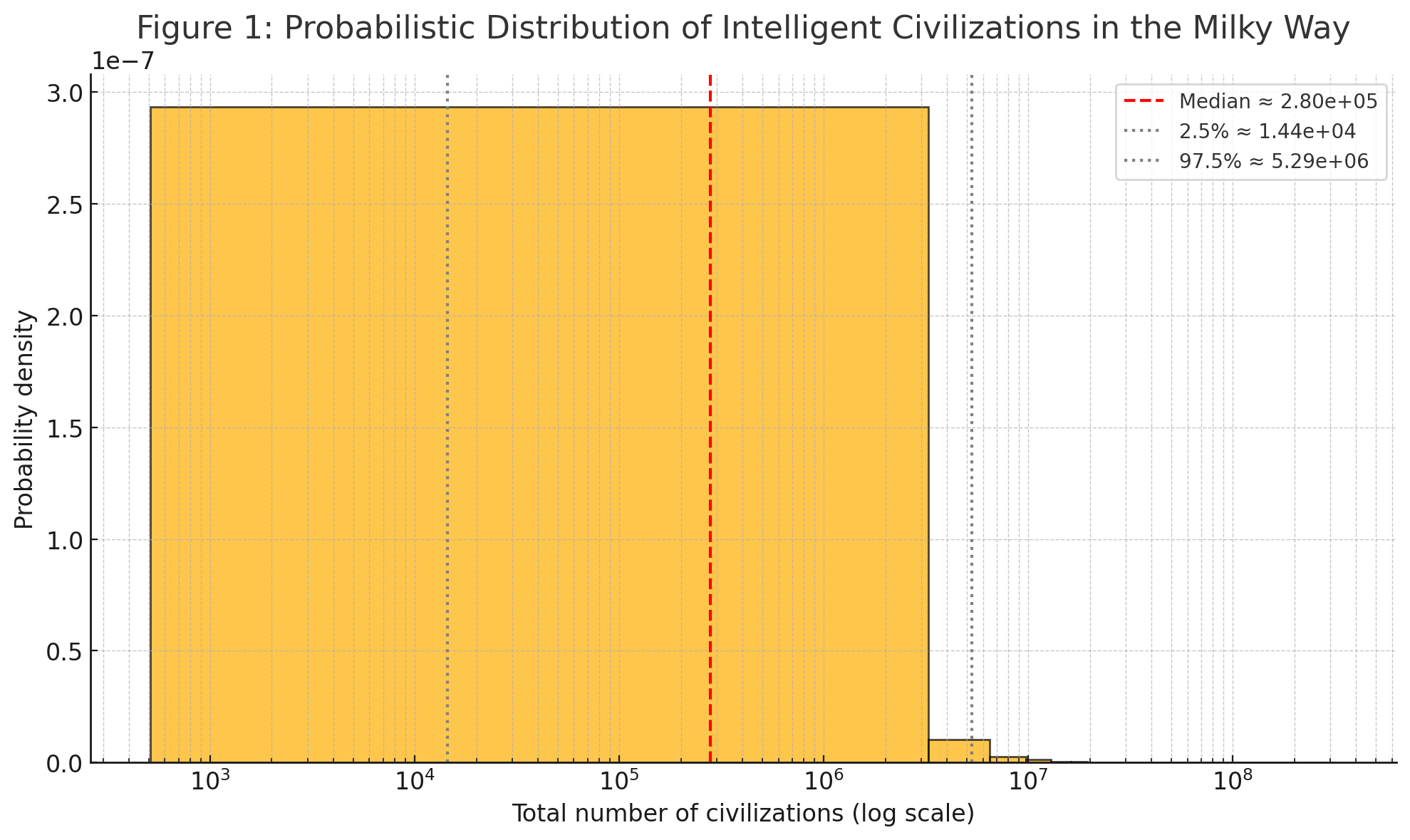
Sensitivity analysis reveals that uncertainty is dominated by:

1. Life emergence probability (f_l): 42% of variance
2. Intelligence evolution probability (f_i): 37% of variance
3. Habitable planet frequency (n_e): 11% of variance

This highlights that our estimates remain primarily constrained by our profound uncertainty about life’s emergence and the evolution of intelligence, rather than by astronomical parameters.

4.2 Earth’s Developmental Trajectory

For Earth’s future trajectory over the next 1,000 years, our simulations project three main outcomes with approximately equal probabilities:

Table 4: Earth Civilization Trajectory (10,000 Monte Carlo runs)

| Outcome | Probability | 95% Confidence Interval |
|---------|------------|------------------------|
| Sustained development | 32% | (20%, 44%) |
| Technological plateau | 34% | (21%, 47%) |
| Systemic decline | 34% | (20%, 48%) |

This distribution reflects high uncertainty rather than a prediction of doom - each pathway remains plausible given current conditions and historical patterns.

Importantly, these outcomes emerge from multiple pathways, not just technological determinism:

• Sustained development: Includes both AI-driven and non-AI futures, ecological balance scenarios, and space expansion
• Technological plateau: Includes both stable equilibria and oscillatory patterns
• Systemic decline: Includes both recoverable setbacks and more severe collapses

4.3 Contact Probabilities

Our model suggests interstellar contact through various mechanisms remains improbable within the next 1,000 years, but with significant uncertainty:

Table 5: Contact Probability Estimates

| Contact Type | Median Probability | 95% CI |
|-------------|-------------------|--------|
| Radio signal detection | 0.02% | (0.001%, 0.5%) |
| Technosignature detection | 0.1% | (0.005%, 2%) |
| Physical probe detection | 0.05% | (0.002%, 1.5%) |
| Direct contact | <0.001% | (<0.0001%, 0.01%) |

These low probabilities stem from multiple factors: spatial separation, civilizational lifespans, detection limitations, and the diversity of potential developmental pathways that may not prioritize expansion or communication.

5. Alternative Explanations and Models

We explicitly acknowledge competing frameworks for understanding intelligent life and civilizational development:

5.1 The Rare Earth Hypothesis

Ward and Brownlee (2000) argue that complex life requires an improbable combination of astronomical, geological, and biological factors. Their model suggests that while microbial life may be common, intelligence might be exceptionally rare. Key differences from our model:

• Places greater emphasis on early evolutionary bottlenecks
• Focuses on Earth-specific contingencies in multicellular evolution
• Projects far fewer technological civilizations (<100 in the galaxy)

5.2 Non-Expansion Models

Several theorists (Sagan, Cirkovic, Brin) have proposed that advanced civilizations may not prioritize expansion or communication. Possibilities include:

• Conservation ethics: Advanced societies may value non-interference
• Simulation focus: Civilizations might turn inward toward virtual realms
• Efficiency imperatives: Communication might use channels unknown to us

These alternatives highlight that technological advancement need not follow Earth-centric assumptions about space exploration or broadcasting.

5.3 Great Filter Theories

Hanson’s “Great Filter” concept suggests one or more extremely improbable steps in civilizational evolution. Our model incorporates this possibility through low-probability transitions, but acknowledges alternative filter placements:

• Behind us: Abiogenesis or eukaryotic evolution might be the main filter
• Ahead of us: Technological maturity challenges might doom most civilizations
• Distributed: Multiple moderate filters rather than a single great one

6. Limitations and Uncertainties

We explicitly acknowledge several fundamental limitations:

1. Sample size of one: All projections about civilizational evolution extrapolate from Earth’s single example
2. Parameter uncertainty: Critical parameters remain radically uncertain despite our best efforts
3. Anthropic observation bias: Current conditions might be unrepresentative of cosmic norms
4. Model structure uncertainty: Our framework makes strong assumptions about civilizational dynamics
5. Validation challenges: Historical data provides only limited testing for long-term projections

Given these limitations, all conclusions should be interpreted as exploratory rather than definitive, and multiple competing models should be considered simultaneously.

7. Conclusion

Our Metakinetics framework represents an attempt to move beyond static probabilistic models of civilizational evolution toward a more dynamic, systems-based approach. While this offers potential advantages in capturing feedback loops and multiple developmental pathways, we emphasize that all such modeling remains highly speculative.

The key findings – the likely existence but rarity of other intelligence, the approximately equal probabilities of different futures for Earth, and the low likelihood of contact – should be interpreted not as predictions but as structured explorations of possibility space given current knowledge.

The most robust conclusion is meta-level: our profound uncertainty about key parameters means that confident assertions about civilizational futures or extraterrestrial life remain premature. The primary value of this work lies not in any specific numerical estimate, but in providing a more rigorous framework for exploring these questions as new data emerges.

Addendum

Sociokinetics was expanded into Metakinetics to establish a more generalizable ontological framework for modeling dynamic systems composed of interacting agents and macro-level forces. Whereas Sociokinetics was developed with a focus on human societies, emphasizing political institutions, civic behavior, and cultural transitions, Metakinetics abstracts these structures to accommodate a broader range of systems, including non-human, artificial, and natural phenomena.

Metakinetics enables the simulation of any system in which structured interactions give rise to emergent behavior over time. This occurs through formalizing agents, forces, and state transitions as modular and domain-agnostic components.

This generalization of Metakinetics extends the applicability of the framework beyond sociopolitical analysis toward universal modeling of complex adaptive systems.